Plasticity of von Mises

This tutorial aims to demonstrate an efficient implementation of the plasticity model of von Mises using an external operator defining the elastoplastic constitutive relations written with the help of the 3rd-party package Numba. Here we consider a cylinder expansion problem in the two-dimensional case in a symmetric formulation.

This tutorial is based on the original implementation of the problem via legacy FEniCS 2019 and its extension for the modern FEniCSx in the setting of convex optimization. A detailed conclusion of the von Mises plastic model in the case of the cylinder expansion problem can be found in [Bonnet et al., 2014]. Do not hesitate to visit the mentioned sources for more information.

We assume the knowledge of the return-mapping procedure, commonly used in the solid mechanics community to solve elastoplasticity problems.

Notation

Denoting the displacement vector \(\boldsymbol{u}\) we define the strain tensor \(\boldsymbol{\varepsilon}\) as follows

\[ \boldsymbol{\varepsilon} = \frac{1}{2}\left( \nabla\boldsymbol{u} + \nabla\boldsymbol{u}^T \right). \]

Throughout the tutorial, we stick to the Mandel-Voigt notation, according to which the stress tensor \(\boldsymbol{\sigma}\) and the strain tensor \(\boldsymbol{\varepsilon}\) are written as 4-size vectors with the following components

\[\begin{align*} & \boldsymbol{\sigma} = [\sigma_{xx}, \sigma_{yy}, \sigma_{zz}, \sqrt{2}\sigma_{xy}]^T, \\ & \boldsymbol{\varepsilon} = [\varepsilon_{xx}, \varepsilon_{yy}, \varepsilon_{zz}, \sqrt{2}\varepsilon_{xy}]^T. \end{align*}\]

Denoting the deviatoric operator \(\mathrm{dev}\), we introduce two additional quantities of interest: the cumulative plastic strain \(p\) and the equivalent stress \(\sigma_\text{eq}\) defined by the following formulas:

\[\begin{align*} & p = \sqrt{\frac{2}{3} \boldsymbol{e} \cdot \boldsymbol{e}}, \\ & \sigma_\text{eq} = \sqrt{\frac{3}{2}\boldsymbol{s} \cdot \boldsymbol{s}}, \end{align*}\]

where \(\boldsymbol{e} = \mathrm{dev}\boldsymbol{\varepsilon}\) and \(\boldsymbol{s} = \mathrm{dev}\boldsymbol{\sigma}\) are deviatoric parts of the stain and stress tensors respectively.

Problem formulation

The domain of the problem \(\Omega\) represents the first quarter of the hollow cylinder with inner \(R_i\) and outer \(R_o\) radii, where symmetry conditions are set on the left and bottom sides and pressure is set on the inner wall \(\partial\Omega_\text{inner}\). The behaviour of cylinder material is defined by the von Mises yield criterion \(f\) with the linear isotropic hardening law (3)

(3)\[ f(\boldsymbol{\sigma}) = \sigma_\text{eq}(\boldsymbol{\sigma}) - \sigma_0 - Hp \leq 0, \]

where \(\sigma_0\) is a uniaxial strength and \(H\) is an isotropic hardening modulus, which is defined through the Young modulus \(E\) and the tangent elastic modulus \(E_t = \frac{EH}{E+H}\).

Let V be the functional space of admissible displacement fields. Then, the weak formulation of this problem can be written as follows:

Find \(\boldsymbol{u} \in V\) such that

(4)\[ F(\boldsymbol{u}; \boldsymbol{v}) = \int\limits_\Omega \boldsymbol{\sigma}(\boldsymbol{\varepsilon}(\boldsymbol{u})) \cdot \boldsymbol{\varepsilon(v)} \,\mathrm{d}\boldsymbol{x} - F_\text{ext}(\boldsymbol{v}) = 0, \quad \forall \boldsymbol{v} \in V. \]

The external force \(F_{\text{ext}}(\boldsymbol{v})\) represents the pressure inside the cylinder and is written as the following Neumann condition

\[ F_\text{ext}(\boldsymbol{v}) = \int\limits_{\partial\Omega_\text{inner}} (-q \boldsymbol{n}) \cdot \boldsymbol{v} \,\mathrm{d}\boldsymbol{x}, \]

where the vector \(\boldsymbol{n}\) is the outward normal to the cylinder surface and the loading parameter \(q\) is progressively adjusted from 0 to \(q_\text{lim} = \frac{2}{\sqrt{3}}\sigma_0\log\left(\frac{R_o}{R_i}\right)\), the analytical collapse load for the perfect plasticity model without hardening.

The modelling is performed under assumptions of the plane strain and an associative plasticity law.

In this tutorial, we treat the stress tensor \(\boldsymbol{\sigma}\) as an external operator acting on the strain tensor \(\boldsymbol{\varepsilon}(\boldsymbol{u})\) and represent it through a FEMExternalOperator object. By the implementation of this external operator, we mean an implementation of the return-mapping procedure, the most common approach to solve plasticity problems. With the help of this procedure, we compute both values of the stress tensor \(\boldsymbol{\sigma}\) and its derivative, so-called the tangent moduli \(\boldsymbol{C}_\text{tang}\).

As before, in order to solve the nonlinear equation (4) we need to compute the Gateaux derivative of \(F\) in the direction \(\boldsymbol{\hat{u}} \in V\):

\[ J(\boldsymbol{u}; \boldsymbol{\hat{u}},\boldsymbol{v}) := D_{\boldsymbol{u}} [F(\boldsymbol{u}; \boldsymbol{v})]\{\boldsymbol{\hat{u}}\} := \int\limits_\Omega \left( \boldsymbol{C}_\text{tang}(\boldsymbol{\varepsilon}(\boldsymbol{u})) \cdot \boldsymbol{\varepsilon}(\boldsymbol{\hat{u}}) \right) \cdot \boldsymbol{\varepsilon(v)} \,\mathrm{d}\boldsymbol{x}, \quad \forall \boldsymbol{v} \in V. \]

The advantage of the von Mises model is that the return-mapping procedure may be performed analytically, so the stress tensor and the tangent moduli may be expressed explicitly using any package. In our case, we the Numba library to define the behaviour of the external operator and its derivative.

Implementation

Preamble

from mpi4py import MPI  # noqa: F401
from petsc4py import PETSc

import matplotlib.pyplot as plt
import numba
import numpy as np
from demo_plasticity_von_mises_pure_ufl import plasticity_von_mises_pure_ufl
from utilities import build_cylinder_quarter, find_cell_by_point

import basix
import ufl
from dolfinx import fem
from dolfinx.fem.petsc import NonlinearProblem
from dolfinx.nls.petsc import NewtonSolver
from dolfinx_external_operator import (
    FEMExternalOperator,
    evaluate_external_operators,
    evaluate_operands,
    replace_external_operators,
)

Here we define geometrical and material parameters of the problem as well as some useful constants.

R_e, R_i = 1.3, 1.0  # external/internal radius

E, nu = 70e3, 0.3  # elastic parameters
E_tangent = E / 100.0  # tangent modulus
H = E * E_tangent / (E - E_tangent)  # hardening modulus
sigma_0 = 250.0  # yield strength

lmbda = E * nu / (1.0 + nu) / (1.0 - 2.0 * nu)
mu = E / 2.0 / (1.0 + nu)
# stiffness matrix
C_elas = np.array(
    [
        [lmbda + 2.0 * mu, lmbda, lmbda, 0.0],
        [lmbda, lmbda + 2.0 * mu, lmbda, 0.0],
        [lmbda, lmbda, lmbda + 2.0 * mu, 0.0],
        [0.0, 0.0, 0.0, 2.0 * mu],
    ],
    dtype=PETSc.ScalarType,
)

deviatoric = np.eye(4, dtype=PETSc.ScalarType)
deviatoric[:3, :3] -= np.full((3, 3), 1.0 / 3.0, dtype=PETSc.ScalarType)

mesh, facet_tags, facet_tags_labels = build_cylinder_quarter()

k_u = 2
V = fem.functionspace(mesh, ("Lagrange", k_u, (mesh.geometry.dim,)))
# Boundary conditions
bottom_facets = facet_tags.find(facet_tags_labels["Lx"])
left_facets = facet_tags.find(facet_tags_labels["Ly"])

bottom_dofs_y = fem.locate_dofs_topological(V.sub(1), mesh.topology.dim - 1, bottom_facets)
left_dofs_x = fem.locate_dofs_topological(V.sub(0), mesh.topology.dim - 1, left_facets)

sym_bottom = fem.dirichletbc(np.array(0.0, dtype=PETSc.ScalarType), bottom_dofs_y, V.sub(1))
sym_left = fem.dirichletbc(np.array(0.0, dtype=PETSc.ScalarType), left_dofs_x, V.sub(0))

bcs = [sym_bottom, sym_left]


def epsilon(v):
    grad_v = ufl.grad(v)
    return ufl.as_vector([grad_v[0, 0], grad_v[1, 1], 0, np.sqrt(2.0) * 0.5 * (grad_v[0, 1] + grad_v[1, 0])])


k_stress = 2 * (k_u - 1)
ds = ufl.Measure(
    "ds",
    domain=mesh,
    subdomain_data=facet_tags,
    metadata={"quadrature_degree": k_stress, "quadrature_scheme": "default"},
)

dx = ufl.Measure(
    "dx",
    domain=mesh,
    metadata={"quadrature_degree": k_stress, "quadrature_scheme": "default"},
)

Du = fem.Function(V, name="displacement_increment")
S_element = basix.ufl.quadrature_element(mesh.topology.cell_name(), degree=k_stress, value_shape=(4,))
S = fem.functionspace(mesh, S_element)
sigma = FEMExternalOperator(epsilon(Du), function_space=S)

n = ufl.FacetNormal(mesh)
loading = fem.Constant(mesh, PETSc.ScalarType(0.0))

v = ufl.TestFunction(V)
F = ufl.inner(sigma, epsilon(v)) * dx - ufl.inner(loading * -n, v) * ds(facet_tags_labels["inner"])

# Internal state
P_element = basix.ufl.quadrature_element(mesh.topology.cell_name(), degree=k_stress)
P = fem.functionspace(mesh, P_element)

p = fem.Function(P, name="cumulative_plastic_strain")
dp = fem.Function(P, name="incremental_plastic_strain")
sigma_n = fem.Function(S, name="stress_n")

Defining the external operator

During the automatic differentiation of the form \(F\), the following terms will appear in the Jacobian

\[ \frac{\mathrm{d} \boldsymbol{\sigma}}{\mathrm{d} \boldsymbol{\varepsilon}}(\boldsymbol{\varepsilon}(\boldsymbol{u})) \cdot \boldsymbol{\varepsilon}(\boldsymbol{\hat{u}}) = \boldsymbol{C}_\text{tang}(\boldsymbol{\varepsilon}(\boldsymbol{u})) \cdot \boldsymbol{\varepsilon}(\boldsymbol{\hat{u}}), \]

where the “trial” part \(\boldsymbol{\varepsilon}(\boldsymbol{\hat{u}})\) will be handled by the framework and the derivative of the operator \(\frac{\mathrm{d} \boldsymbol{\sigma}}{\mathrm{d} \boldsymbol{\varepsilon}}\) must be implemented by the user. In this tutorial, we implement the derivative using the Numba package.

First of all, we implement the return-mapping procedure locally in the function _kernel. It computes the values of the stress tensor, the tangent moduli and the increment of cumulative plastic strain at a single Gausse node. For more details, visit the original implementation of this problem for the legacy FEniCS 2019.

Then we iterate over each Gauss node and compute the quantities of interest globally in the return_mapping function with the @numba.njit decorator. This guarantees that the function will be compiled during its first call and ordinary for-loops will be efficiently processed.

num_quadrature_points = P_element.dim


@numba.njit
def return_mapping(deps_, sigma_n_, p_):
    """Performs the return-mapping procedure."""
    num_cells = deps_.shape[0]

    C_tang_ = np.empty((num_cells, num_quadrature_points, 4, 4), dtype=PETSc.ScalarType)
    sigma_ = np.empty_like(sigma_n_)
    dp_ = np.empty_like(p_)

    def _kernel(deps_local, sigma_n_local, p_local):
        """Performs the return-mapping procedure locally."""
        sigma_elastic = sigma_n_local + C_elas @ deps_local
        s = deviatoric @ sigma_elastic
        sigma_eq = np.sqrt(3.0 / 2.0 * np.dot(s, s))

        f_elastic = sigma_eq - sigma_0 - H * p_local
        f_elastic_plus = (f_elastic + np.sqrt(f_elastic**2)) / 2.0

        dp = f_elastic_plus / (3 * mu + H)

        n_elas = s / sigma_eq * f_elastic_plus / f_elastic
        beta = 3 * mu * dp / sigma_eq

        sigma = sigma_elastic - beta * s

        n_elas_matrix = np.outer(n_elas, n_elas)
        C_tang = C_elas - 3 * mu * (3 * mu / (3 * mu + H) - beta) * n_elas_matrix - 2 * mu * beta * deviatoric

        return C_tang, sigma, dp

    for i in range(0, num_cells):
        for j in range(0, num_quadrature_points):
            C_tang_[i, j], sigma_[i, j], dp_[i, j] = _kernel(deps_[i, j], sigma_n_[i, j], p_[i, j])

    return C_tang_, sigma_, dp_

Now nothing stops us from defining the implementation of the external operator derivative (the tangent tensor \(\boldsymbol{C}_\text{tang}\)) in the function C_tang_impl. It returns global values of the derivative, stress tensor and the cumulative plastic increment.

def C_tang_impl(deps):
    num_cells = deps.shape[0]
    num_quadrature_points = int(deps.shape[1] / 4)

    deps_ = deps.reshape((num_cells, num_quadrature_points, 4))
    sigma_n_ = sigma_n.x.array.reshape((num_cells, num_quadrature_points, 4))
    p_ = p.x.array.reshape((num_cells, num_quadrature_points))

    C_tang_, sigma_, dp_ = return_mapping(deps_, sigma_n_, p_)

    return C_tang_.reshape(-1), sigma_.reshape(-1), dp_.reshape(-1)

It is worth noting that at the time of the derivative evaluation, we compute the values of the external operator as well. Thus, there is no need for a separate implementation of the operator \(\boldsymbol{\sigma}\). We will reuse the output of the C_tang_impl to update values of the external operator further in the Newton loop.

def sigma_external(derivatives):
    if derivatives == (1,):
        return C_tang_impl
    else:
        return NotImplementedError


sigma.external_function = sigma_external

Note

The framework allows implementations of external operators and its derivatives to return additional outputs. In our example, alongside with the values of the derivative, the function C_tang_impl returns, the values of the stress tensor and the cumulative plastic increment. Both additional outputs may be reused by the user afterwards in the Newton loop.

Form manipulations

As in the previous tutorials before solving the problem we need to perform some transformation of both linear and bilinear forms.

u_hat = ufl.TrialFunction(V)
J = ufl.derivative(F, Du, u_hat)
J_expanded = ufl.algorithms.expand_derivatives(J)

F_replaced, F_external_operators = replace_external_operators(F)
J_replaced, J_external_operators = replace_external_operators(J_expanded)

F_form = fem.form(F_replaced)
J_form = fem.form(J_replaced)

Note

We remind that in the code above we replace FEMExternalOperator objects by their fem.Function representatives, the coefficients which are allocated during the call of the FEMExternalOperator constructor. The access to these coefficients may be carried out through the field ref_coefficient of an FEMExternalOperator object. For example, the following code returns the finite coefficient associated with the tangent matrix C_tang = J_external_operators[0].ref_coefficient.

Variables initialization and compilation

Before assembling the forms, we have to initialize the external operators. In particular, the tangent matrix should be equal to the elastic one during the first loading step, so to initialize the former, we evaluate external operators for a close-to-zero displacement field.

Solving the problem

u = fem.Function(V, name="displacement")


class PlasticityProblem(NonlinearProblem):
    def form(self, x: PETSc.Vec) -> None:
        """This function is called before the residual or Jacobian is
        computed. This is usually used to update ghost values, but here
        we also use it to evaluate the external operators.

        Args:
           x: The vector containing the latest solution
        """
        # The following line is from the standard NonlinearProblem class
        x.ghostUpdate(addv=PETSc.InsertMode.INSERT, mode=PETSc.ScatterMode.FORWARD)

        evaluated_operands = evaluate_operands(F_external_operators)
        ((_, sigma_new, dp_new),) = evaluate_external_operators(J_external_operators, evaluated_operands)

        # This avoids having to evaluate the external operators of F.
        sigma.ref_coefficient.x.array[:] = sigma_new
        dp.x.array[:] = dp_new


problem = PlasticityProblem(F_replaced, Du, bcs=bcs, J=J_replaced)

x_point = np.array([[R_i, 0, 0]])
cells, points_on_process = find_cell_by_point(mesh, x_point)

q_lim = 2.0 / np.sqrt(3.0) * np.log(R_e / R_i) * sigma_0
num_increments = 20
load_steps = np.linspace(0, 1.1, num_increments, endpoint=True) ** 0.5
loadings = q_lim * load_steps
results = np.zeros((num_increments, 2))

solver = NewtonSolver(mesh.comm, problem)
solver.max_it = 200
solver.rtol = 1e-8
ksp = solver.krylov_solver
opts = PETSc.Options()  # type: ignore
option_prefix = ksp.getOptionsPrefix()
opts[f"{option_prefix}ksp_type"] = "preonly"
opts[f"{option_prefix}pc_type"] = "lu"
opts[f"{option_prefix}pc_factor_mat_solver_type"] = "mumps"
ksp.setFromOptions()

eps = np.finfo(PETSc.ScalarType).eps

for i, loading_v in enumerate(loadings):
    loading.value = loading_v
    Du.x.array[:] = eps

    solver.solve(Du)

    u.x.petsc_vec.axpy(1.0, Du.x.petsc_vec)
    u.x.scatter_forward()

    p.x.petsc_vec.axpy(1.0, dp.x.petsc_vec)
    sigma_n.x.array[:] = sigma.ref_coefficient.x.array

    if len(points_on_process) > 0:
        results[i, :] = (u.eval(points_on_process, cells)[0], loading.value / q_lim)

Post-processing

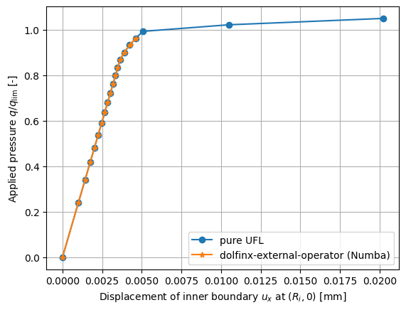
In order to verify the correctness of obtained results, we perform their comparison against a “pure UFl” implementation. Thanks to simplicity of the von Mises model we can express stress tensor and tangent moduli analytically within the variational setting and so in UFL. Such a performant implementation is presented by the function plasticity_von_mises_pure_ufl.

results_pure_ufl = plasticity_von_mises_pure_ufl(verbose=False)

Here below we plot the displacement of the inner boundary of the cylinder \(u_x(R_i, 0)\) with respect to the applied pressure in the von Mises model with isotropic hardening. The plastic deformations are reached at the pressure \(q_{\lim}\) equal to the analytical collapse load for perfect plasticity.

if len(points_on_process) > 0:
    plt.plot(results_pure_ufl[:, 0], results_pure_ufl[:, 1], "o-", label="pure UFL")
    plt.plot(results[:, 0], results[:, 1], "*-", label="dolfinx-external-operator (Numba)")
    plt.xlabel(r"Displacement of inner boundary $u_x$ at $(R_i, 0)$ [mm]")
    plt.ylabel(r"Applied pressure $q/q_{\text{lim}}$ [-]")
    plt.legend()
    plt.grid()
    plt.savefig("output.png")
    plt.show()

References

[BFR14]

Marc Bonnet, Attilio Frangi, and Christian Rey. The finite element method in solid mechanics. McGraw Hill Education, 2014. URL: https://hal.science/hal-01083772.