Hyperelasticity via Input-Convex Neural Networks (ICNN) (PyTorch)

This tutorial demonstrates how to define a complex hyperelastic constitutive model using PyTorch automatic differentiation (AD) and integrate it with FEniCSx. In solid mechanics, standard models (like Neo-Hookean) have simple analytical derivatives. However, data-driven constitutive equations (like neural network surrogates) require automatic differentiation to evaluate stresses and tangent operators (Jacobians) at the quadrature points of the finite element mesh.

Here, we stick to the Isihara hyperelasticity model [Isihara et al., 1951]. The tutorial is based on the work of Thakolkaran et al. [2022] on unsupervised deep-learning hyperelasticity without stress data (NN-EUCLID): EUCLID-code/EUCLID-hyperelasticity-NN.

To get familiarized with hyperelasticity problems, we recommend first taking a look at the following basic tutorials:

• Numerical Tours of Computational Mechanics with FEniCSx by Jérémy Bleyer.

• The FEniCSx tutorial by Jørgen S. Dokken and Garth N. Wells.

Problem Formulation

We solve a hyperelasticity boundary value problem on a 2D square domain \(\Omega\) containing elliptic holes, subjected to displacement-controlled tensile loading.

Let \(V\) be the functional space of admissible displacement fields. Under the assumption of quasi-static displacement-controlled loading and in the absence of body forces, the weak formulation of the equilibrium equation is expressed as follows.

Find \(\mathbf{u} \in V\) satisfying the Dirichlet boundary conditions such that:

\[ F(\mathbf{u}; \mathbf{v}) = \int\limits_\Omega \mathbf{P}(\mathbf{F}) : \nabla\mathbf{v} \, \mathrm{d}\mathbf{x} = 0, \quad \forall \mathbf{v} \in V_0 \]

where:

• \(\mathbf{F} = \mathbf{I} + \nabla\mathbf{u}\) is the deformation gradient.

• \(\mathbf{P}(\mathbf{F}) = \frac{\partial W}{\partial \mathbf{F}}\) is the first Piola-Kirchhoff stress tensor derived from the strain energy density \(W(\mathbf{F})\).

• \(\mathbf{v} \in V_0\) is a test function vanishing on the Dirichlet boundaries.

Implementation

Preamble

from mpi4py import MPI

from utilities import build_square_with_elliptic_holes

import basix
import dolfinx.plot
import ufl
from dolfinx import default_scalar_type, fem, mesh
from dolfinx.fem.petsc import NonlinearProblem

# Define external function for Piola-Kirchhoff stress and its derivative
from dolfinx_external_operator import (
    FEMExternalOperator,
    evaluate_external_operators,
    evaluate_operands,
    replace_external_operators,
)
from dolfinx_external_operator.petsc import assemble_residual_with_callback

# isort: split

from functools import partial

import matplotlib.pyplot as plt
import numpy as np
import pyvista
import torch
import torch.func

Geometry and boundary conditions

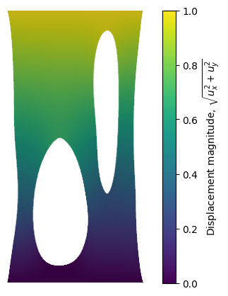
We solve a 2D tension problem of a square specimen with elliptic holes. The boundary conditions consist of zero displacement at the bottom, and a prescribed vertical displacement at the top. We use quadratic Lagrange elements for the displacement field \(\mathbf{u}\).

L = 1.0  # Length
W = 1.0  # Height

domain, facet_tags, facet_tags_labels = build_square_with_elliptic_holes(L=L, lc=0.02)
V = fem.functionspace(domain, ("Lagrange", 2, (domain.geometry.dim,)))


def bottom(x):
    return np.isclose(x[1], 0.0)


def top(x):
    return np.isclose(x[1], W)


fdim = domain.topology.dim - 1
bottom_facets = mesh.locate_entities_boundary(domain, fdim, bottom)
top_facets = mesh.locate_entities_boundary(domain, fdim, top)

marked_facets = np.hstack([bottom_facets, top_facets])
marked_values = np.hstack([np.full_like(bottom_facets, 1), np.full_like(top_facets, 2)])
sorted_facets = np.argsort(marked_facets)
facet_tag = mesh.meshtags(domain, fdim, marked_facets[sorted_facets], marked_values[sorted_facets])

bottom_dofs = fem.locate_dofs_topological(V, facet_tag.dim, facet_tag.find(1))
top_dofs_uy = fem.locate_dofs_topological(V.sub(1), facet_tag.dim, facet_tag.find(2))
top_dofs_ux = fem.locate_dofs_topological(V.sub(0), facet_tag.dim, facet_tag.find(2))
u_D_bottom = np.array((0,) * domain.geometry.dim, dtype=default_scalar_type)
u_D_top = fem.Constant(domain, 0.0)

bcs_u = [
    fem.dirichletbc(u_D_top, top_dofs_uy, V.sub(1)),
    fem.dirichletbc(fem.Constant(domain, 0.0), top_dofs_ux, V.sub(0)),
    fem.dirichletbc(u_D_bottom, bottom_dofs, V),
]

Constitutive Formulation

We model the hyperelastic response using an Input-Convex Neural Network (ICNN) designed to output a strain energy density \(W(\mathbf{F})\) that is convex with respect to the right Cauchy-Green strain invariants. Objectivity is satisfied by expressing \(W\) as a function of the right Cauchy-Green deformation tensor \(\mathbf{C} = \mathbf{F}^T\mathbf{F}\).

Following [Thakolkaran et al., 2022], the strain energy density is formulated as:

\[ W(\mathbf{F}) = W_{\mathbf{Q}, \mathbf{\mathcal{A}}}^{\text{NN}}(\mathbf{E}(\mathbf{F})) + W^0 + \mathbf{H}:\mathbf{E}, \]

where:

• \(\mathbf{E} = \frac{1}{2}(\mathbf{C} - \mathbf{I})\) is the Green-Lagrange strain tensor, representing the deformation.

• \(W_{\mathbf{Q}, \mathbf{\mathcal{A}}}^{\text{NN}}(\mathbf{E})\) is the neural network mapping the strain tensor \(\mathbf{E}\) (via its invariants) to a scalar energy.

• \(W^0\) is a scalar correction offsetting the energy density to zero in the reference configuration:

\[ W^0 = -\left. W_{\mathbf{Q}, \mathbf{\mathcal{A}}}^{\text{NN}}(\mathbf{E}(\mathbf{F})) \right|_{\mathbf{F} = \mathbf{I}} \]

• \(\mathbf{H}\) is a stress correction tensor ensuring that the stress vanishes in the undeformed state (\(\mathbf{F}=\mathbf{I}\)):

\[ \mathbf{H} = -\left. \frac{\partial W_{\mathbf{Q}, \mathbf{\mathcal{A}}}^{\text{NN}}(\mathbf{E})}{\partial \mathbf{F}} \right|_{\mathbf{F}=\mathbf{I}} \]

The first Piola-Kirchhoff stress \(\mathbf{P}\) is computed as:

\[ \mathbf{P}(\mathbf{F}) = \frac{\partial W(\mathbf{F})}{\partial \mathbf{F}} = \mathbf{P}^\text{NN} + \mathbf{F}\mathbf{H}, \]

where \(\mathbf{P}^\text{NN} := \frac{\partial W^{\text{NN}}}{\partial \mathbf{F}}\) and the tangent modulus is:

\[ \mathbb{C}_{ijkl} = \frac{\partial P_{ij}(\mathbf{F})}{\partial F_{kl}} = \mathbb{C}^\text{NN}_{ijkl} + \delta_{ik} H_{lj} ,\]

where \(\mathbb{C}^\text{NN}_{ijkl} := \frac{\partial^2 W^{\text{NN}}}{\partial F_{ij} \partial F_{kl}}\).

We will load a pre-trained network modeling the Isihara material behaviour to evaluate the strain energy density \(W^{\text{NN}}\). Then, using PyTorch automatic differentiation (AD) tools, we will compute the values of the first Piola-Kirchhoff stress \(\mathbf{P}\) and the tangent \(\mathbb{C}\). The programs resulting from AD will then be used to define the external operators associated with \(\mathbf{P}(\mathbf{F})\) and \(\mathbb{C}\) respectively.

Input-Convex Neural Network (ICNN) in PyTorch

We preserve the same structure of convexLinear and ICNN as defined in the original implementation using custom layers that enforce positive weights in the hidden layers to maintain input-convexity.

Here below, we represent the \(2 \times 2\) tensors \(\mathbf{F}, \mathbf{P}\), and \(\mathbf{H}\) in flattened vector forms, e.g.

\[ \mathbf{P} = [P_{11}, P_{12}, P_{21}, P_{22}]^T .\]

class convexLinear(torch.nn.Module):
    """Custom linear layer with positive weights and no bias"""

    def __init__(
        self,
        size_in,
        size_out,
    ):
        super().__init__()
        self.size_in, self.size_out = size_in, size_out
        weights = torch.Tensor(size_out, size_in)
        self.weights = torch.nn.Parameter(weights)

        # initialize weights
        torch.nn.init.kaiming_uniform_(self.weights, a=np.sqrt(5))

    def forward(self, x):
        w_times_x = torch.mm(x, torch.nn.functional.softplus(self.weights.t()))
        return w_times_x


class ICNN(torch.nn.Module):
    def __init__(self, n_input, n_hidden, n_output, dropout):
        super().__init__()
        # Create Module dicts for the hidden and skip-connection layers
        self.layers = torch.nn.ModuleDict()
        self.skip_layers = torch.nn.ModuleDict()
        self.depth = len(n_hidden)
        self.dropout = dropout[0]
        self.p_dropout = dropout[1]

        self.layers[str(0)] = torch.nn.Linear(n_input, n_hidden[0]).float()
        # Create NN with number of elements in n_hidden as depth
        for i in range(1, self.depth):
            self.layers[str(i)] = convexLinear(n_hidden[i - 1], n_hidden[i]).float()
            self.skip_layers[str(i)] = torch.nn.Linear(n_input, n_hidden[i]).float()

        self.layers[str(self.depth)] = convexLinear(n_hidden[self.depth - 1], n_output).float()
        self.skip_layers[str(self.depth)] = convexLinear(n_input, n_output).float()

    def forward(self, x):
        # Get F components
        F11 = x[:, 0:1]
        F12 = x[:, 1:2]
        F21 = x[:, 2:3]
        F22 = x[:, 3:4]

        # Compute right Cauchy green strain Tensor
        C11 = F11**2 + F21**2
        C12 = F11 * F12 + F21 * F22
        C21 = F11 * F12 + F21 * F22
        C22 = F12**2 + F22**2

        # Compute strain invariants
        I1 = C11 + C22 + 1.0
        I2 = C11 + C22 - C12 * C21 + C11 * C22
        I3 = C11 * C22 - C12 * C21

        # Apply transformation to invariants
        K1 = I1 * torch.pow(I3, -1 / 3) - 3.0
        K2 = I2 * torch.pow(I3, -2 / 3) - 3.0
        J = torch.sqrt(I3)
        K3 = (J - 1) ** 2

        # Concatenate feature
        x_input = torch.cat((K1, K2, K3), 1).float()

        z = x_input.clone()
        z = self.layers[str(0)](z)
        for layer in range(1, self.depth):
            skip = self.skip_layers[str(layer)](x_input)
            z = self.layers[str(layer)](z)
            z += skip
            z = torch.nn.functional.softplus(z)
            z = 1 / 12.0 * torch.square(z)
            if self.training:
                if self.dropout:
                    z = torch.nn.functional.dropout(z, p=self.p_dropout)
        y = self.layers[str(self.depth)](z) + self.skip_layers[str(self.depth)](x_input)
        return y


n_input = 3
n_output = 1
n_hidden = [64, 64, 64]
dropout = [True, 0.2]
model = ICNN(n_input=n_input, n_hidden=n_hidden, n_output=n_output, dropout=dropout)

Once the structure of the ICNN model is defined we can load a pretrained one. In particular, we explore the Isihara model [Isihara et al., 1951] with high noise.

model.load_state_dict(torch.load("Isihara_noise=high.pth"))
model.eval()

ICNN(
  (layers): ModuleDict(
    (0): Linear(in_features=3, out_features=64, bias=True)
    (1): convexLinear()
    (2): convexLinear()
    (3): convexLinear()
  )
  (skip_layers): ModuleDict(
    (1): Linear(in_features=3, out_features=64, bias=True)
    (2): Linear(in_features=3, out_features=64, bias=True)
    (3): convexLinear()
  )
)

Train your own ICNN model!

Here we are not studying how to train the ICNN model. Instead, we load the pretrained one Isihara_noise=high.pth. If you wish to explore other hyperelastic models we encourage you to follow the instructions in the original repository of EUCLID, which we outline here

In the folder with demo_hyperelasticity.py, clone EUCLID-hyperelasticity-NN

git clone https://github.com/EUCLID-code/EUCLID-hyperelasticity-NN

Install pandas and other dependencies, if needed

pip install pandas

Train a new model

cd drivers/
python main.py Isihara high

Note

Although we rely here on the CPU-based PyTorch installation, it is motivated by keeping the external operators demos light. For training of new models, we suggest to install the normal GPU-based PyTorch package.

Then in the code above try

model.load_state_dict(torch.load("Isihara_noise=high.pth"))
model.eval()

Note

There is a bug related to NumPy>=2.0 in EUCLID-hyperelasticity-NN. If the error persists, try this fork with a fix.

PyTorch-based Tangent and Stress Evaluation

We first precompute the constant stress correction tensor \(\mathbf{H}\) and the constant tangent correction \(\mathbb{C}^\text{cor}_{ijkl} = \frac{\partial \mathbf{P}^{\text{cor}}_{ij}}{\partial \mathbf{F}_{kl}} = \delta_{ik} H_{lj}\), since they do not change throughout the loading.

F_0 = torch.zeros((1, 4))
F_0[:, 0] = 1
F_0[:, 3] = 1

F_0.requires_grad = True
W_NN_0 = model(F_0)
P_NN_0 = torch.autograd.grad(W_NN_0, F_0, torch.ones_like(W_NN_0), create_graph=True)[0].squeeze()

# Precompute correction matrix H for stress correction
H_flat = -P_NN_0.detach()
H = torch.tensor(
    [
        [H_flat[0], H_flat[1], 0, 0],
        [H_flat[2], H_flat[3], 0, 0],
        [0, 0, H_flat[0], H_flat[1]],
        [0, 0, H_flat[2], H_flat[3]],
    ],
    dtype=P_NN_0.dtype,
    device=P_NN_0.device,
)

Secondly, we define the behaviour of the constitutive model locally, at a single Gauss point, and then globally by leveraging the modern (JAX-inspired) PyTorch features such that

1. automatic differentiation (torch.func.jacfwd) to compute \(\mathbb{C}^\text{NN}\),

2. vectorization (torch.func.vmap) to extrapolate the local behaviour onto all Gauss points,

3. and JIT compilation (torch.compile) to speed up computations.

Overall, as you will see later, the workflow is very similar to the previous tutorial using JAX.

Install PyTorch 2.0 or later

To be able to use torch.func.jacfwd, torch.func.vmap and torch.compile, make sure that you use torch=>2.0.

Currently, there is an issue with combining all three together. Compile just model instead.

Since PyTorch compiler Inductor currently has tracing limitations when directly compiling nested higher-order functional AD operators (vmap / jacfwd), we compile the underlying neural network model itself instead. This avoids compiler-level limitations while capturing the bulk of the compilation speedup, since the neural network evaluations dominate the computational cost.

# JIT-compile the model to optimize forward and backward passes
model = torch.compile(model)

Now we apply AD and vectorize the functions that compute the stress state. The final dP_dF_impl computes both the stress state and the tangent at all Gauss points at once.

# Define vectorized stress and tangent computation using torch.func


def compute_stress_local(F_single):
    # F_single: shape (4,)
    # Define local energy function for the neural network
    def energy_fn(f):
        return model(f.unsqueeze(0)).squeeze()

    # Stress from neural network (first derivative)
    P_NN = torch.func.grad(energy_fn)(F_single)

    # Stress correction P_cor = F_single @ H (using flat matrix multiplication for efficiency)
    P_cor = F_single @ H.to(F_single)

    P = P_NN + P_cor
    # Return stress as primary output and as auxiliary data
    return P, P


# Vectorize the tangent evaluation over the batch dimension using jacfwd
# with has_aux=True returns a tuple of (tangent, auxiliary_stress)
vectorized_stress_and_tangent = torch.func.vmap(torch.func.jacfwd(compute_stress_local, has_aux=True), in_dims=(0,))


def dP_dF_impl(Fvals):
    F = torch.from_numpy(np.ascontiguousarray(Fvals)).reshape(-1, 4)  # NumPy-compatible without copy
    # Evaluate stress and tangent simultaneously in a single vectorized pass
    dP, P = vectorized_stress_and_tangent(F)

    return dP.reshape(-1).detach().numpy(), P.reshape(-1).detach().numpy()

Similarly to the previous tutorials with plasticity, we do not implement explicitly the evaluation of the stress. Instead, we obtain its values during the evaluation of its derivative and then update the values of the operator in the main Newton loop. This happens because automatic differentiation may evaluate the value of a function while computing its derivative.

FEniCSx Integration of PyTorch model via External Operators

The stress state has one operand, which is the strain tensor \(\mathbf{F}\) (defined as gradU) that depends on the displacement field \(\mathbf{u}\). Here we define both of them and the quadrature space Q, where the external operator will live.

u = fem.Function(V)
v = ufl.TestFunction(V)
d = len(u)
gradU = ufl.variable(ufl.Identity(d) + ufl.grad(u))  # F tensor

# Create a quadrature element and function space for tensor-valued P
quadrature_degree = 2
cell_name = domain.topology.cell_name()
Qe = basix.ufl.quadrature_element(cell_name, value_shape=(d, d), degree=quadrature_degree, scheme="default")
Q = fem.functionspace(domain, Qe)

Finally, we wrap the PyTorch execution code into a Python callable, P_external, and define a FEMExternalOperator that can be used to define the variational formulation.

def P_external(derivatives):
    if derivatives == (1,):
        return dP_dF_impl
    else:
        raise NotImplementedError(f"No external function is defined for the requested derivative {derivatives}.")


P = FEMExternalOperator(gradU, function_space=Q, external_function=P_external)

Note

We don’t need to cover the case if derivatives == (0,) for just calling evaluation of P because, as previously mentioned, thanks to AD we can compute the values of P while computing its derivative. Yet, we still need to properly update the values of P, which will be done in constitutive_update, a function defined below when setting up the nonlinear solver.

Variational Forms

We define the weak form using UFL as usual, compute its directional derivative, and replace it with the replace_external_operators function to allow DOLFINx to assemble the forms.

metadata = {"quadrature_degree": 2}
dx = ufl.Measure("dx", domain=domain, metadata=metadata)

u_hat = ufl.TrialFunction(V)
F = ufl.inner(ufl.grad(v), P) * dx
J = ufl.derivative(F, u, u_hat)

F_replaced, F_external_operators = replace_external_operators(F)
J_replaced, J_external_operators = replace_external_operators(J)

F_form = fem.form(F_replaced)
J_form = fem.form(J_replaced)

Solving the Problem

We set up the PETSc SNES solver using a Newton solver, wrapping the constitutive update in a callback function. This function affects the performance the most, since it will be called on every single iteration of the Newton solver to update the values of \(\mathbf{P}\) and \(\mathbb{C}\).

def constitutive_update(
    F_external_operators: list[FEMExternalOperator],
    J_external_operators: list[FEMExternalOperator],
):
    """Update the constitutive model by evaluating the external operators."""
    evaluated_operands = evaluate_operands(F_external_operators)
    # `dP_dF_impl` will be called here
    ((_, P_new),) = evaluate_external_operators(J_external_operators, evaluated_operands)
    # manually update the values of the external operator
    P.ref_coefficient.x.array[:] = P_new


petsc_options = {
    "snes_type": "vinewtonrsls",
    "snes_linesearch_type": "basic",
    "ksp_type": "preonly",
    "pc_type": "lu",
    "pc_factor_mat_solver_type": "mumps",
    "snes_atol": 1.0e-7,
    "snes_rtol": 1.0e-7,
    "snes_max_it": 50,
    "snes_monitor": "",
}

problem = NonlinearProblem(
    F_replaced, u, J=J_replaced, bcs=bcs_u, petsc_options_prefix="demo_hyperelasticity_", petsc_options=petsc_options
)

assemble_residual_with_callback_ = partial(
    assemble_residual_with_callback,
    problem.u,
    problem.F,
    problem.J,
    bcs_u,
    constitutive_update,  # external callback with respect to SNES
    [F_external_operators, J_external_operators],  # input arguments of the callback
)
problem.solver.setFunction(assemble_residual_with_callback_, problem.b)

We incrementally apply a displacement-controlled tensile load by moving the top boundary.

# Apply a tensile load by incrementally increasing displacement on the top edge
n_steps = 5
max_displacement = 1.0
u.name = "displacement"
u.x.array[:] = 0
for step in range(1, n_steps + 1):
    u_D_top.value = step * max_displacement / n_steps  # moving the top boundary
    problem.solve()
    converged = problem.solver.getConvergedReason()
    num_its = problem.solver.getIterationNumber()
    assert converged, f"Newton solver did not converge at step {step}"
    u.x.scatter_forward()
    if domain.comm.rank == 0:
        print(f"Step {step}: Displacement {u_D_top.value:.2f}, Newton its: {num_its}")

  0 SNES Function norm 2.299854996250e+01

  1 SNES Function norm 1.363018555179e-01

  2 SNES Function norm 2.026796459191e-02

  3 SNES Function norm 1.388250692408e-03

  4 SNES Function norm 9.049586383685e-06

  5 SNES Function norm 2.382180480125e-08
Step 1: Displacement 0.20, Newton its: 5
  0 SNES Function norm 2.046041602712e+01

  1 SNES Function norm 5.912822757409e-02

  2 SNES Function norm 4.474706688376e-03

  3 SNES Function norm 2.232946963379e-05

  4 SNES Function norm 8.304854891383e-08
Step 2: Displacement 0.40, Newton its: 4
  0 SNES Function norm 1.942664282615e+01

  1 SNES Function norm 3.917439365577e-02

  2 SNES Function norm 1.072204688480e-03

  3 SNES Function norm 7.128956208834e-07
Step 3: Displacement 0.60, Newton its: 3
  0 SNES Function norm 1.925033484516e+01

  1 SNES Function norm 2.936954103413e-02

  2 SNES Function norm 4.058528830493e-04

  3 SNES Function norm 3.277502440258e-07
Step 4: Displacement 0.80, Newton its: 3
  0 SNES Function norm 1.964419646783e+01

  1 SNES Function norm 2.454940072366e-02

  2 SNES Function norm 1.894643674790e-04

  3 SNES Function norm 5.023524640166e-07
Step 5: Displacement 1.00, Newton its: 3

Visualize the deformed configuration of the specimen.

try:
    import matplotlib.cm as mcm
    import matplotlib.colors as mcolors
    import pyvista

    import dolfinx.plot

    plotter = pyvista.Plotter(window_size=[600, 400], off_screen=True)
    topology, cell_types, x = dolfinx.plot.vtk_mesh(V)
    grid = pyvista.UnstructuredGrid(topology, cell_types, x)
    vals = np.zeros((x.shape[0], 3))
    vals[:, : len(u)] = u.x.array.reshape((x.shape[0], len(u)))
    grid["u"] = vals

    # Calculate displacement magnitude
    mag = np.linalg.norm(vals[:, : len(u)], axis=1)
    grid["mag"] = mag

    warped = grid.warp_by_vector("u", factor=1)
    plotter.add_mesh(warped, scalars="mag", cmap="viridis", show_edges=False, show_scalar_bar=False)
    plotter.view_xy()
    plotter.camera.tight()
    image = plotter.screenshot(None, transparent_background=True, return_img=True)

    fig, ax = plt.subplots(figsize=(7, 5))
    ax.imshow(image)
    ax.axis("off")

    # Create matching colorbar using matplotlib
    norm = mcolors.Normalize(vmin=mag.min(), vmax=mag.max())
    smap = mcm.ScalarMappable(cmap="viridis", norm=norm)
    smap.set_array([])
    fig.colorbar(smap, ax=ax, label=r"Displacement magnitude, $\sqrt{u_x^2 + u_y^2}$")

    fig.savefig("displacement_nn.png", bbox_inches="tight", dpi=200, transparent=True)
    plt.show()

except ImportError:
    print("pyvista required for this plot")

2026-07-14 19:08:53.407 (  10.900s) [    7F38AE693140]vtkXOpenGLRenderWindow.:1460  WARN| bad X server connection. DISPLAY=:99.0

Verification against UFL-based formulation

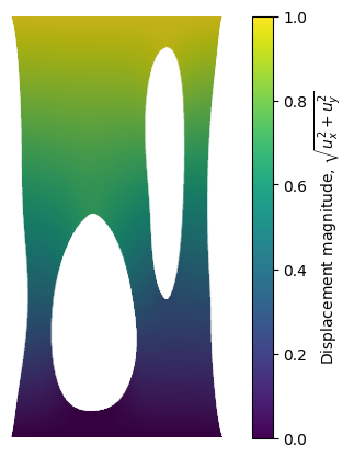
To verify the results obtained with the ICNN model wrapped via external operators, we implement a pure UFL version of the Isihara model.

The variational formulation of the baseline problem is:

Find \(\mathbf{u}_{\text{UFL}} \in V\) satisfying the Dirichlet boundary conditions such that:

\[ F_{\text{UFL}}(\mathbf{u}_{\text{UFL}}; \mathbf{v}) = \int\limits_\Omega \mathbf{P}(\mathbf{F}) : \nabla\mathbf{v} \, \mathrm{d}\mathbf{x} = 0, \quad \forall \mathbf{v} \in V_0 \]

where the stress tensor is evaluated symbolically via \(\mathbf{P}(\mathbf{F}) = \frac{\partial W_{\text{Isihara}}}{\partial \mathbf{F}}\) using UFL’s automatic differentiation tool ufl.diff.

The strain energy density function \(W_{\text{Isihara}}(\mathbf{F})\) is defined explicitly as:

\[ W_{\text{Isihara}}(\mathbf{F}) = 0.5(\bar{I}_1 - 3) + (\bar{I}_2 - 3) + (\bar{I}_1 - 3)^2 + 1.5(J - 1)^2 \]

where the deviatoric invariants \(\bar{I}_1\) and \(\bar{I}_2\) are:

• \(\bar{I}_1 = J^{-2/3} I_1\)

• \(\bar{I}_2 = J^{-4/3} I_2\)

• \(J = \det(\mathbf{F})\) is the volume ratio (determinant of the deformation gradient tensor \(\mathbf{F}\)).

• \(I_1 = \text{tr}(\mathbf{C}) = \text{tr}(\mathbf{F}^T\mathbf{F}) + 1.0\) and \(I_2 = I_1 + J^2 - 1.0\) under the 2D plane strain assumption.

The UFL formulation is very straightforward.

u_UFL = fem.Function(V)
v = ufl.TestFunction(V)
d = len(u_UFL)
# Deformation gradient
F_ = ufl.variable(ufl.Identity(d) + ufl.grad(u_UFL))

C = F_.T * F_
J_ = ufl.det(F_)
I1 = ufl.tr(C) + 1.0
I2 = I1 + J_**2 - 1.0

# Isihara model parameters
I1_bar = (J_ ** (-2.0 / 3.0)) * I1
I2_bar = (J_ ** (-4.0 / 3.0)) * I2

W_Isihara = 0.5 * (I1_bar - 3.0) + (I2_bar - 3.0) + (I1_bar - 3.0) ** 2 + 1.5 * (J_ - 1.0) ** 2

P = ufl.diff(W_Isihara, F_)

F_UFL = ufl.inner(ufl.grad(v), P) * dx

We could then explicitly apply ufl.derivative to F_UFL to obtain the Jacobian J_UFL but this will be done automatically in NonlinearProblem under the hood.

Now we simply define the nonlinear problem with the same petsc_options as before and solve the UFL-based problem.

problem_UFL = NonlinearProblem(
    F_UFL, u_UFL, bcs=bcs_u, petsc_options=petsc_options, petsc_options_prefix="UFL_hyperelasticity_"
)

# Apply a tensile load by incrementally increasing displacement on the top edge
u_UFL.name = "UFL_displacement"
u_UFL.x.array[:] = 0
for step in range(1, n_steps + 1):
    u_D_top.value = step * max_displacement / n_steps
    problem_UFL.solve()
    converged = problem_UFL.solver.getConvergedReason()
    num_its = problem_UFL.solver.getIterationNumber()
    assert converged, f"Newton solver did not converge at step {step}"
    u_UFL.x.scatter_forward()
    if domain.comm.rank == 0:
        print(f"Step {step}: Displacement {u_D_top.value:.3f}, Newton its: {num_its}")

  0 SNES Function norm 2.292306829596e+01
  1 SNES Function norm 1.384425829962e-01
  2 SNES Function norm 2.165757538978e-02

  3 SNES Function norm 1.598857382931e-03
  4 SNES Function norm 1.265191909729e-05

  5 SNES Function norm 9.278222025453e-10
Step 1: Displacement 0.200, Newton its: 5
  0 SNES Function norm 2.019102641988e+01
  1 SNES Function norm 5.486152659117e-02
  2 SNES Function norm 3.538812074121e-03

  3 SNES Function norm 1.123056133459e-05
  4 SNES Function norm 2.227936895925e-10
Step 2: Displacement 0.400, Newton its: 4
  0 SNES Function norm 1.915189434457e+01
  1 SNES Function norm 3.420010110614e-02
  2 SNES Function norm 6.303355267404e-04

  3 SNES Function norm 2.904576083877e-07
Step 3: Displacement 0.600, Newton its: 3
  0 SNES Function norm 1.924203421618e+01
  1 SNES Function norm 2.481539966717e-02

  2 SNES Function norm 2.075532643710e-04
  3 SNES Function norm 3.917187363408e-08
Step 4: Displacement 0.800, Newton its: 3
  0 SNES Function norm 2.008297557314e+01

  1 SNES Function norm 1.855060914390e-02
  2 SNES Function norm 9.207464065142e-05
  3 SNES Function norm 9.125901251798e-09
Step 5: Displacement 1.000, Newton its: 3

try:
    import matplotlib.cm as mcm
    import matplotlib.colors as mcolors
    import pyvista

    import dolfinx.plot

    plotter = pyvista.Plotter(window_size=[600, 400], off_screen=True)
    topology, cell_types, x = dolfinx.plot.vtk_mesh(V)
    grid = pyvista.UnstructuredGrid(topology, cell_types, x)
    vals = np.zeros((x.shape[0], 3))
    vals[:, : len(u_UFL)] = u_UFL.x.array.reshape((x.shape[0], len(u_UFL)))
    grid["u"] = vals

    # Calculate displacement magnitude
    mag = np.linalg.norm(vals[:, : len(u_UFL)], axis=1)
    grid["mag"] = mag

    warped = grid.warp_by_vector("u", factor=1)
    plotter.add_mesh(warped, scalars="mag", cmap="viridis", show_edges=False, show_scalar_bar=False)
    plotter.view_xy()
    plotter.camera.tight()
    image = plotter.screenshot(None, transparent_background=True, return_img=True)

    fig, ax = plt.subplots(figsize=(7, 5))
    ax.imshow(image)
    ax.axis("off")

    # Create matching colorbar using matplotlib
    norm = mcolors.Normalize(vmin=mag.min(), vmax=mag.max())
    smap = mcm.ScalarMappable(cmap="viridis", norm=norm)
    smap.set_array([])
    fig.colorbar(smap, ax=ax, label=r"Displacement magnitude, $\sqrt{u_x^2 + u_y^2}$")

    fig.savefig("displacement_ufl.png", bbox_inches="tight", dpi=200, transparent=True)
    plt.show()

except ImportError:
    print("pyvista required for this plot")

Comparison of Deformed Configurations

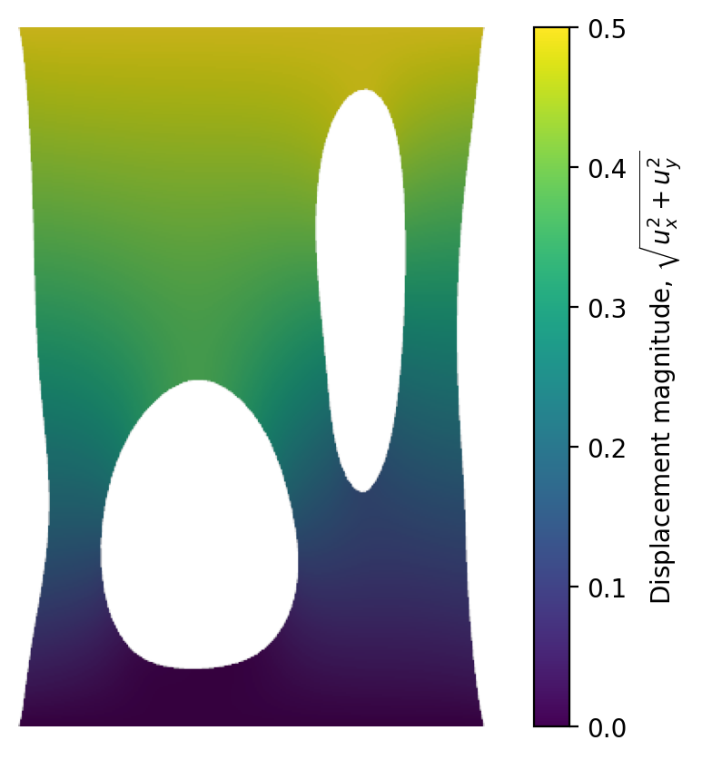
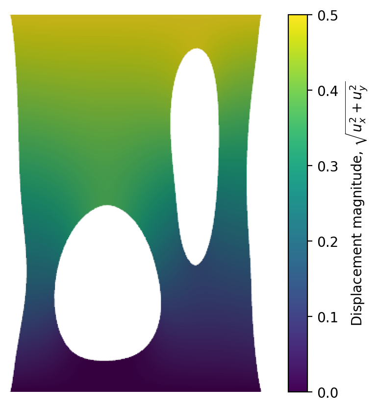
Below, we compare the deformed configuration predicted by the Neural Network external operator against the analytical UFL baseline.

Neural Network Operator

UFL-based formulation

Error Analysis

To quantitatively assess the difference between the Input-Convex Neural Network (ICNN) external operator and the analytical UFL baseline, we compute two error metrics at the end of the simulation:

1. Relative Maximum Nodal Displacement Error (relative \(L^\infty\) norm):

\[ e_{\infty, \text{rel}} = \frac{\max_i |u_i - u_{\text{UFL}, i}|}{\max_i |u_{\text{UFL}, i}|} \]

np.abs(u.x.array[:] - u_UFL.x.array[:]).max() / np.abs(u_UFL.x.array[:]).max()

np.float64(0.0016946183833891626)

2. Absolute \(L^2\) Displacement Difference:

\[ e_{L^2} = \sqrt{\int\limits_\Omega (\mathbf{u} - \mathbf{u}_{\text{UFL}})^2 \, \mathrm{d}\mathbf{x}} \]

np.sqrt(MPI.COMM_WORLD.allreduce(fem.assemble_scalar(fem.form((u - u_UFL) ** 2 * dx)), op=MPI.SUM))

np.float64(0.0006879071121988283)

Errors look quite promising :)

References

[IHT51] (1,2)

Akira Isihara, Natsuki Hashitsume, and Masao Tatibana. Statistical theory of rubber-like elasticity. v. (two-dimensional stretching). The Journal of Chemical Physics, 19(12):1508–1512, 1951. doi:10.1063/1.1748111.

[TJZ+22] (1,2)

Prakash Thakolkaran, Akshay Joshi, Yiwen Zheng, Moritz Flaschel, Laura De Lorenzis, and Siddhant Kumar. NN-EUCLID: Deep-learning hyperelasticity without stress data. Journal of the Mechanics and Physics of Solids, 169:1–29, 2022. doi:10.1016/j.jmps.2022.105076.