Plasticity of von Mises

This tutorial aims to demonstrate an efficient implementation of the plasticity model of von Mises using an external operator defining the elastoplastic constitutive relations written with the help of the 3rd-party package Numba. Here we consider a cylinder expansion problem in the two-dimensional case in a symmetric formulation.

This tutorial is based on the original implementation of the problem via legacy FEniCS 2019 and its extension for the modern FEniCSx in the setting of convex optimization. A detailed conclusion of the von Mises plastic model in the case of the cylinder expansion problem can be found in [Bonnet et al., 2014]. Do not hesitate to visit the mentioned sources for more information.

We assume the knowledge of the return-mapping procedure, commonly used in the solid mechanics community to solve elastoplasticity problems.

Notation

Denoting the displacement vector \(\boldsymbol{u}\) we define the strain tensor \(\boldsymbol{\varepsilon}\) as follows

\[ \boldsymbol{\varepsilon} = \frac{1}{2}\left( \nabla\boldsymbol{u} + \nabla\boldsymbol{u}^T \right). \]

Throughout the tutorial, we stick to the Mandel-Voigt notation, according to which the stress tensor \(\boldsymbol{\sigma}\) and the strain tensor \(\boldsymbol{\varepsilon}\) are written as 4-size vectors with the following components

\[\begin{align*} & \boldsymbol{\sigma} = [\sigma_{xx}, \sigma_{yy}, \sigma_{zz}, \sqrt{2}\sigma_{xy}]^T, \\ & \boldsymbol{\varepsilon} = [\varepsilon_{xx}, \varepsilon_{yy}, \varepsilon_{zz}, \sqrt{2}\varepsilon_{xy}]^T. \end{align*}\]

Denoting the deviatoric operator \(\mathrm{dev}\), we introduce two additional quantities of interest: the cumulative plastic strain \(p\) and the equivalent stress \(\sigma_\text{eq}\) defined by the following formulas:

\[\begin{align*} & p = \sqrt{\frac{2}{3} \boldsymbol{e} \cdot \boldsymbol{e}}, \\ & \sigma_\text{eq} = \sqrt{\frac{3}{2}\boldsymbol{s} \cdot \boldsymbol{s}}, \end{align*}\]

where \(\boldsymbol{e} = \mathrm{dev}\boldsymbol{\varepsilon}\) and \(\boldsymbol{s} = \mathrm{dev}\boldsymbol{\sigma}\) are deviatoric parts of the stain and stress tensors respectively.

Problem formulation

The domain of the problem \(\Omega\) represents the first quarter of the hollow cylinder with inner \(R_i\) and outer \(R_o\) radii, where symmetry conditions are set on the left and bottom sides and pressure is set on the inner wall \(\partial\Omega_\text{inner}\). The behaviour of cylinder material is defined by the von Mises yield criterion \(f\) with the linear isotropic hardening law (3)

(3)\[ f(\boldsymbol{\sigma}) = \sigma_\text{eq}(\boldsymbol{\sigma}) - \sigma_0 - Hp \leq 0, \]

where \(\sigma_0\) is a uniaxial strength and \(H\) is an isotropic hardening modulus, which is defined through the Young modulus \(E\) and the tangent elastic modulus \(E_t = \frac{EH}{E+H}\).

Let V be the functional space of admissible displacement fields. Then, the weak formulation of this problem can be written as follows:

Find \(\boldsymbol{u} \in V\) such that

(4)\[ F(\boldsymbol{u}; \boldsymbol{v}) = \int\limits_\Omega \boldsymbol{\sigma}(\boldsymbol{\varepsilon}(\boldsymbol{u})) \cdot \boldsymbol{\varepsilon(v)} \mathrm{d}\boldsymbol{x} - F_\text{ext}(\boldsymbol{v}) = 0, \quad \forall \boldsymbol{v} \in V. \]

The external force \(F_{\text{ext}}(\boldsymbol{v})\) represents the pressure inside the cylinder and is written as the following Neumann condition

\[ F_\text{ext}(\boldsymbol{v}) = q \int\limits_{\partial\Omega_\text{inner}} \boldsymbol{n} \cdot \boldsymbol{v} d\boldsymbol{x}, \]

where the vector \(\boldsymbol{n}\) is a normal to the cylinder surface and the loading parameter \(q\) is progressively increased from 0 to \(q_\text{lim} = \frac{2}{\sqrt{3}}\sigma_0\log\left(\frac{R_o}{R_i}\right)\), the analytical collapse load for the perfect plasticity model without hardening.

The modelling is performed under assumptions of the plane strain and an associative plasticity law.

In this tutorial, we treat the stress tensor \(\boldsymbol{\sigma}\) as an external operator acting on the strain tensor \(\boldsymbol{\varepsilon}(\boldsymbol{u})\) and represent it through a FEMExternalOperator object. By the implementation of this external operator, we mean an implementation of the return-mapping procedure, the most common approach to solve plasticity problems. With the help of this procedure, we compute both values of the stress tensor \(\boldsymbol{\sigma}\) and its derivative, so-called the tangent stiffness matrix \(\boldsymbol{C}_\text{tang}\).

As before, in order to solve the nonlinear equation (4) we need to compute the Gateaux derivative of \(F\) in the direction \(\boldsymbol{\hat{u}} \in V\):

\[ J(\boldsymbol{u}; \boldsymbol{\hat{u}},\boldsymbol{v}) := D_{\boldsymbol{u}} [F(\boldsymbol{u}; \boldsymbol{v})]\{\boldsymbol{\hat{u}}\} := \int\limits_\Omega \left( \boldsymbol{C}_\text{tang}(\boldsymbol{\varepsilon}(\boldsymbol{u})) \cdot \boldsymbol{\varepsilon}(\boldsymbol{\hat{u}}) \right) \cdot \boldsymbol{\varepsilon(v)} \mathrm{d}\boldsymbol{x}, \quad \forall \boldsymbol{v} \in V. \]

The advantage of the von Mises model is that the return-mapping procedure may be performed analytically, so the stress tensor and the tangent stiffness matrix may be expressed explicitly using any package. In our case, we the Numba library to define the behaviour of the external operator and its derivative.

Implementation

Preamble

from mpi4py import MPI
from petsc4py import PETSc

import matplotlib.pyplot as plt
import numba
import numpy as np
from plasticity_von_mises_pure_ufl import plasticity_von_mises_interpolation, plasticity_von_mises_pure_ufl
from solvers import LinearProblem
from utilities import build_cylinder_quarter, find_cell_by_point

import basix
import ufl
from dolfinx import common, fem
from dolfinx_external_operator import (
    FEMExternalOperator,
    evaluate_external_operators,
    evaluate_operands,
    replace_external_operators,
)

Here we define geometrical and material parameters of the problem as well as some useful constants.

R_e, R_i = 1.3, 1.0  # external/internal radius

E, nu = 70e3, 0.3  # elastic parameters
E_tangent = E / 100.0  # tangent modulus
H = E * E_tangent / (E - E_tangent)  # hardening modulus
sigma_0 = 250.0  # yield strength

lmbda = E * nu / (1.0 + nu) / (1.0 - 2.0 * nu)
mu = E / 2.0 / (1.0 + nu)
# stiffness matrix
C_elas = np.array(
    [
        [lmbda + 2.0 * mu, lmbda, lmbda, 0.0],
        [lmbda, lmbda + 2.0 * mu, lmbda, 0.0],
        [lmbda, lmbda, lmbda + 2.0 * mu, 0.0],
        [0.0, 0.0, 0.0, 2.0 * mu],
    ],
    dtype=PETSc.ScalarType,
)

deviatoric = np.eye(4, dtype=PETSc.ScalarType)
deviatoric[:3, :3] -= np.full((3, 3), 1.0 / 3.0, dtype=PETSc.ScalarType)

mesh, facet_tags, facet_tags_labels = build_cylinder_quarter()

k_u = 2
V = fem.functionspace(mesh, ("Lagrange", k_u, (2,)))
# Boundary conditions
bottom_facets = facet_tags.find(facet_tags_labels["Lx"])
left_facets = facet_tags.find(facet_tags_labels["Ly"])

bottom_dofs_y = fem.locate_dofs_topological(V.sub(1), mesh.topology.dim - 1, bottom_facets)
left_dofs_x = fem.locate_dofs_topological(V.sub(0), mesh.topology.dim - 1, left_facets)

sym_bottom = fem.dirichletbc(np.array(0.0, dtype=PETSc.ScalarType), bottom_dofs_y, V.sub(1))
sym_left = fem.dirichletbc(np.array(0.0, dtype=PETSc.ScalarType), left_dofs_x, V.sub(0))

bcs = [sym_bottom, sym_left]


def epsilon(v):
    grad_v = ufl.grad(v)
    return ufl.as_vector([grad_v[0, 0], grad_v[1, 1], 0, np.sqrt(2.0) * 0.5 * (grad_v[0, 1] + grad_v[1, 0])])


k_stress = 2 * (k_u - 1)
ds = ufl.Measure(
    "ds",
    domain=mesh,
    subdomain_data=facet_tags,
    metadata={"quadrature_degree": k_stress, "quadrature_scheme": "default"},
)

dx = ufl.Measure(
    "dx",
    domain=mesh,
    metadata={"quadrature_degree": k_stress, "quadrature_scheme": "default"},
)

Du = fem.Function(V, name="displacement_increment")
S_element = basix.ufl.quadrature_element(mesh.topology.cell_name(), degree=k_stress, value_shape=(4,))
S = fem.functionspace(mesh, S_element)
sigma = FEMExternalOperator(epsilon(Du), function_space=S)

n = ufl.FacetNormal(mesh)
loading = fem.Constant(mesh, PETSc.ScalarType(0.0))

v = ufl.TestFunction(V)
F = ufl.inner(sigma, epsilon(v)) * dx - loading * ufl.inner(v, n) * ds(facet_tags_labels["inner"])

# Internal state
P_element = basix.ufl.quadrature_element(mesh.topology.cell_name(), degree=k_stress, value_shape=())
P = fem.functionspace(mesh, P_element)

p = fem.Function(P, name="cumulative_plastic_strain")
dp = fem.Function(P, name="incremental_plastic_strain")
sigma_n = fem.Function(S, name="stress_n")

Defining the external operator

During the automatic differentiation of the form \(F\), the following terms will appear in the Jacobian

\[ \frac{\mathrm{d} \boldsymbol{\sigma}}{\mathrm{d} \boldsymbol{\varepsilon}}(\boldsymbol{\varepsilon}(\boldsymbol{u})) \cdot \boldsymbol{\varepsilon}(\boldsymbol{\hat{u}}) = \boldsymbol{C}_\text{tang}(\boldsymbol{\varepsilon}(\boldsymbol{u})) \cdot \boldsymbol{\varepsilon}(\boldsymbol{\hat{u}}), \]

where the “trial” part \(\boldsymbol{\varepsilon}(\boldsymbol{\hat{u}})\) will be handled by the framework and the derivative of the operator \(\frac{\mathrm{d} \boldsymbol{\sigma}}{\mathrm{d} \boldsymbol{\varepsilon}}\) must be implemented by the user. In this tutorial, we implement the derivative using the Numba package.

First of all, we implement the return-mapping procedure locally in the function _kernel. It computes the values of the stress tensor, the tangent stiffness matrix and the increment of cumulative plastic strain at a single Gausse node. For more details, visit the original implementation of this problem for the legacy FEniCS 2019.

Then we iterate over each Gauss node and compute the quantities of interest globally in the return_mapping function with the @numba.njit decorator. This guarantees that the function will be compiled during its first call and ordinary for-loops will be efficiently processed.

num_quadrature_points = P_element.dim


@numba.njit
def return_mapping(deps_, sigma_n_, p_):
    """Performs the return-mapping procedure."""
    num_cells = deps_.shape[0]

    C_tang_ = np.empty((num_cells, num_quadrature_points, 4, 4), dtype=PETSc.ScalarType)
    sigma_ = np.empty_like(sigma_n_)
    dp_ = np.empty_like(p_)

    def _kernel(deps_local, sigma_n_local, p_local):
        """Performs the return-mapping procedure locally."""
        sigma_elastic = sigma_n_local + C_elas @ deps_local
        s = deviatoric @ sigma_elastic
        sigma_eq = np.sqrt(3.0 / 2.0 * np.dot(s, s))

        f_elastic = sigma_eq - sigma_0 - H * p_local
        f_elastic_plus = (f_elastic + np.sqrt(f_elastic**2)) / 2.0

        dp = f_elastic_plus / (3 * mu + H)

        n_elas = s / sigma_eq * f_elastic_plus / f_elastic
        beta = 3 * mu * dp / sigma_eq

        sigma = sigma_elastic - beta * s

        n_elas_matrix = np.outer(n_elas, n_elas)
        C_tang = C_elas - 3 * mu * (3 * mu / (3 * mu + H) - beta) * n_elas_matrix - 2 * mu * beta * deviatoric

        return C_tang, sigma, dp

    for i in range(0, num_cells):
        for j in range(0, num_quadrature_points):
            C_tang_[i, j], sigma_[i, j], dp_[i, j] = _kernel(deps_[i, j], sigma_n_[i, j], p_[i, j])

    return C_tang_, sigma_, dp_

Now nothing stops us from defining the implementation of the external operator derivative (the stiffness tangent tensor \(\boldsymbol{C}_\text{tang}\)) in the function C_tang_impl. It returns global values of the derivative, stress tensor and the cumulative plastic increment.

def C_tang_impl(deps):
    num_cells = deps.shape[0]
    num_quadrature_points = int(deps.shape[1] / 4)

    deps_ = deps.reshape((num_cells, num_quadrature_points, 4))
    sigma_n_ = sigma_n.x.array.reshape((num_cells, num_quadrature_points, 4))
    p_ = p.x.array.reshape((num_cells, num_quadrature_points))

    C_tang_, sigma_, dp_ = return_mapping(deps_, sigma_n_, p_)

    return C_tang_.reshape(-1), sigma_.reshape(-1), dp_.reshape(-1)

It is worth noting that at the time of the derivative evaluation, we compute the values of the external operator as well. Thus, there is no need for a separate implementation of the operator \(\boldsymbol{\sigma}\). We will reuse the output of the C_tang_impl to update values of the external operator further in the Newton loop.

def sigma_external(derivatives):
    if derivatives == (1,):
        return C_tang_impl
    else:
        return NotImplementedError


sigma.external_function = sigma_external

Note

The framework allows implementations of external operators and its derivatives to return additional outputs. In our example, alongside with the values of the derivative, the function C_tang_impl returns, the values of the stress tensor and the cumulative plastic increment. Both additional outputs may be reused by the user afterwards in the Newton loop.

Form manipulations

As in the previous tutorials before solving the problem we need to perform some transformation of both linear and bilinear forms.

u_hat = ufl.TrialFunction(V)
J = ufl.derivative(F, Du, u_hat)
J_expanded = ufl.algorithms.expand_derivatives(J)

F_replaced, F_external_operators = replace_external_operators(F)
J_replaced, J_external_operators = replace_external_operators(J_expanded)

F_form = fem.form(F_replaced)
J_form = fem.form(J_replaced)

Note

We remind that in the code above we replace FEMExternalOperator objects by their fem.Function representatives, the coefficients which are allocated during the call of the FEMExternalOperator constructor. The access to these coefficients may be carried out through the field ref_coefficient of an FEMExternalOperator object. For example, the following code returns the finite coefficient associated with the tangent matrix C_tang = J_external_operators[0].ref_coefficient.

Variables initialization and compilation

Before assembling the forms, we have to initialize the external operators. In particular, the tangent matrix should be equal to the elastic one during the first loading step, so to initialize the former, we evaluate external operators for a close-to-zero displacement field.

At the same time, we estimate the compilation overhead caused by the first call of JIT-ed Numba functions.

# We need to initialize `Du` with small values in order to avoid the division by
# zero error
eps = np.finfo(PETSc.ScalarType).eps
Du.x.array[:] = eps

timer = common.Timer("DOLFINx_timer")
timer.start()
evaluated_operands = evaluate_operands(F_external_operators)
_ = evaluate_external_operators(J_external_operators, evaluated_operands)
timer.stop()
pass_1 = timer.elapsed()[0]

timer.start()
evaluated_operands = evaluate_operands(F_external_operators)
_ = evaluate_external_operators(J_external_operators, evaluated_operands)
timer.stop()
pass_2 = timer.elapsed()[0]

print(f"\nNumba's JIT compilation overhead: {pass_1 - pass_2}")

Numba's JIT compilation overhead: 3.45

Solving the problem

Solving the problem is carried out in a manually implemented Newton solver.

u = fem.Function(V, name="displacement")
du = fem.Function(V, name="Newton_correction")
external_operator_problem = LinearProblem(J_replaced, F_replaced, Du, bcs=bcs)

# Defining a cell containing (Ri, 0) point, where we calculate a value of u
# In order to run this program in parallel we need capture the process, to which
# this point is attached
x_point = np.array([[R_i, 0, 0]])
cells, points_on_process = find_cell_by_point(mesh, x_point)

q_lim = 2.0 / np.sqrt(3.0) * np.log(R_e / R_i) * sigma_0
num_increments = 20
max_iterations, relative_tolerance = 200, 1e-8
load_steps = (np.linspace(0, 1.1, num_increments, endpoint=True) ** 0.5)[1:]
loadings = q_lim * load_steps
results = np.zeros((num_increments, 2))

for i, loading_v in enumerate(loadings):
    loading.value = loading_v
    external_operator_problem.assemble_vector()

    residual_0 = residual = external_operator_problem.b.norm()
    Du.x.array[:] = 0.0

    if MPI.COMM_WORLD.rank == 0:
        print(f"\nresidual , {residual} \n increment: {i+1!s}, load = {loading.value}")

    for iteration in range(0, max_iterations):
        if residual / residual_0 < relative_tolerance:
            break
        external_operator_problem.assemble_matrix()
        external_operator_problem.solve(du)
        du.x.scatter_forward()

        Du.vector.axpy(-1.0, du.vector)
        Du.x.scatter_forward()

        evaluated_operands = evaluate_operands(F_external_operators)

        # Implementation of an external operator may return several outputs and
        # not only its evaluation. For example, `C_tang_impl` returns a tuple of
        # Numpy-arrays with values of `C_tang`, `sigma` and `dp`.
        ((_, sigma_new, dp_new),) = evaluate_external_operators(J_external_operators, evaluated_operands)

        # In order to update the values of the external operator we may directly
        # access them and avoid the call of
        # `evaluate_external_operators(F_external_operators, evaluated_operands).`
        sigma.ref_coefficient.x.array[:] = sigma_new
        dp.x.array[:] = dp_new

        external_operator_problem.assemble_vector()
        residual = external_operator_problem.b.norm()

        if MPI.COMM_WORLD.rank == 0:
            print(f"    it# {iteration} residual: {residual}")

    u.vector.axpy(1.0, Du.vector)
    u.x.scatter_forward()

    # Taking into account the history of loading
    p.vector.axpy(1.0, dp.vector)
    # skip scatter forward, p is not ghosted.
    sigma_n.x.array[:] = sigma.ref_coefficient.x.array
    # skip scatter forward, sigma is not ghosted.

    if len(points_on_process) > 0:
        results[i + 1, :] = (-u.eval(points_on_process, cells)[0], loading.value / q_lim)

residual , 8.599242028001447 
 increment: 1, load = 18.22357591920427
    it# 0 residual: 2.86659570639356e-13

residual , 3.561922674126921 
 increment: 2, load = 25.772028219874418
    it# 0 residual: 1.1619299386056414e-13

residual , 2.7331593969517707 
 increment: 3, load = 31.564159387650495
    it# 0 residual: 1.0946480970885102e-13

residual , 2.304159956922752 
 increment: 4, load = 36.44715183840854
    it# 0 residual: 8.656123856986615e-14

residual , 2.030005673581492 
 increment: 5, load = 40.74915454846896
    it# 0 residual: 8.168071528973626e-14

residual , 1.8352654137151767 
 increment: 6, load = 44.63846229092138
    it# 0 residual: 7.192300232670426e-14

residual , 1.6877007264469919 
 increment: 7, load = 48.21504988051979
    it# 0 residual: 7.085573696289195e-14

residual , 1.5708735345101743 
 increment: 8, load = 51.544056439748836
    it# 0 residual: 6.593085701564125e-14

residual , 1.4753966797476157 
 increment: 9, load = 54.67072775761281
    it# 0 residual: 6.515849416789851e-14

residual , 1.3954648755256611 
 increment: 10, load = 57.628007017682094
    it# 0 residual: 6.730873016584998e-14

residual , 1.3272683288056422 
 increment: 11, load = 60.44076366255657
    it# 0 residual: 6.544208278137888e-14

residual , 1.268188909824636 
 increment: 12, load = 63.12831877530099
    it# 0 residual: 1.4893010071834571
    it# 1 residual: 0.024011279690787098
    it# 2 residual: 3.0594479646378868e-06
    it# 3 residual: 8.303498067487531e-14

residual , 1.2163598639239093 
 increment: 13, load = 65.70603739900179
    it# 0 residual: 0.8161940858616228
    it# 1 residual: 0.07723280379263806
    it# 2 residual: 9.315749140976803e-06
    it# 3 residual: 4.413515811511117e-13

residual , 1.1704093926445502 
 increment: 14, load = 68.18637745152637
    it# 0 residual: 0.8359673987800559
    it# 1 residual: 0.013714168292272132
    it# 2 residual: 1.815711060675932e-06
    it# 3 residual: 6.968459024152898e-14

residual , 1.1293037097279741 
 increment: 15, load = 70.57960604342466
    it# 0 residual: 1.6640529483784086
    it# 1 residual: 0.821481976652028
    it# 2 residual: 0.002415098137142869
    it# 3 residual: 9.3096662838394e-08
    it# 4 residual: 6.732687003196926e-14

residual , 1.0922469475492926 
 increment: 16, load = 72.89430367681707
    it# 0 residual: 0.6400702322368389
    it# 1 residual: 0.2833799350485556
    it# 2 residual: 0.014196471902242862
    it# 3 residual: 7.2922851684052155e-06
    it# 4 residual: 3.821350105252596e-12

residual , 1.05861506969511 
 increment: 17, load = 75.13772839134165
    it# 0 residual: 1.9811818203618505
    it# 1 residual: 0.050114056098219645
    it# 2 residual: 2.3347429368046748e-05
    it# 3 residual: 1.3031864124389719e-11

residual , 1.0279109246863802 
 increment: 18, load = 77.31608465962326
    it# 0 residual: 7.1610994372466035
    it# 1 residual: 4.26585685457389
    it# 2 residual: 0.6035764966419548
    it# 3 residual: 0.00912868907030283
    it# 4 residual: 1.957348242537754e-06
    it# 5 residual: 5.314889461278251e-13

residual , 0.9997328847209843 
 increment: 19, load = 79.43472582175275
    it# 0 residual: 1.6790196670813418
    it# 1 residual: 0.022175619855480548
    it# 2 residual: 3.371293463438318e-06
    it# 3 residual: 8.554016782829364e-13

Post-processing

results_interpolation = plasticity_von_mises_interpolation(verbose=False)
results_pure_ufl = plasticity_von_mises_pure_ufl(verbose=False)

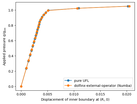
if len(points_on_process) > 0:
    plt.plot(results_pure_ufl[:, 0], results_pure_ufl[:, 1], "-o", label="pure UFL")
    plt.plot(results[:, 0], results[:, 1], "-o", label="dolfinx-external-operator (Numba)")
    # plt.plot(-results_interpolation[:, 0], results_interpolation[:, 1], "-o", label="interpolation")
    plt.xlabel(r"Displacement of inner boundary at $(R_i, 0)$")
    plt.ylabel(r"Applied pressure $q/q_{lim}$")
    plt.legend()
    plt.show()

[BFR14]

Marc Bonnet, Attilio Frangi, and Christian Rey. The finite element method in solid mechanics. McGraw Hill Education, 2014. URL: https://hal.science/hal-01083772.